Retriever Models for Open Domain Question-Answering
It’s a sci-fi staple. A vital component of the legendary Turing test. The dream of many across the world. And, until recently, impossible.
We are talking about the ability to ask a machine a question and receive a genuinely intelligent, insightful answer.
Until recently, technology like this existed only in books, Hollywood, and our collective imagination. Now, it is everywhere. Most of us use this technology every day, and we often don’t even notice it.
Google is just one example. Over the last few years, Google has gradually introduced an intelligent question-answering angle to search. When we now ask how do I tie my shoelaces?" Google gives us the ‘exact answer’ alongside the context or video this answer came from:

We can ask other questions like “Is Google Skynet?" and this time return an even more precise answer “Yes”.
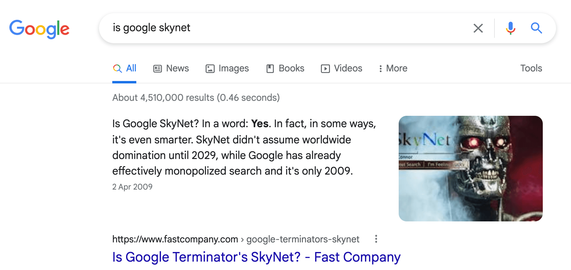
In this example, Google returns an exact answer and the context (paragraph) from where the answer is extracted.
How does Google do this? And more importantly, why should we care?
This search style emulates a human-like interaction. We’re asking a question in natural language as if we were speaking to another person. This natural language Q&A creates a very different search experience to traditional search.
Imagine you find yourself in the world’s biggest warehouse. You have no idea how the place is organized. All you know is that your task is to find some round marble-like objects.
Where do you start? Well, we need to figure out how the warehouse is organized. Maybe everything is stored alphabetically, categorized by industry, or intended use. The traditional search interface requires that we understand how the warehouse is structured before we begin searching. Often, there is a specific ‘query language’ such as:
SELECT * WHERE 'material' == 'marble'

or

("marble" | "stone") & "product"
Our first task is to learn this query language so we can search. Once we understand how the warehouse is structured, we use that knowledge to begin our search. How do we find “round marble-like objects”? We can narrow our search down using similar queries to those above, but we are in the world’s biggest warehouse, so this will take a very long time.
Without a natural Q&A-style interface, this is your search. Unless your users know the ins and outs of the warehouse and its contents, they’re going to struggle.
What happens if we add a natural Q&A-style interface to the warehouse? Imagine we now have people in the warehouse whose entire purpose is to guide us through the warehouse. These people know exactly where everything is.
Those people can understand our question of “where can I find the round marble-like objects?". It may take a few tries until we find the exact object we’re looking for, but we now have a guide that understands our question. There is no longer the need to understand how the warehouse is organized nor to know the exact name of what it is we’re trying to find.
With this natural Q&A-style interface, your users now have a guide. They just need to be able to ask a question.
Answering Questions
How can we design these natural, human-like Q&A interfaces? The answer is open-domain question-answering (ODQA). ODQA allows us to use natural language to query a database.
That means that, given a dataset like a set of internal company documents, online documentation, or as is the case with Google, everything on the world’s internet, we can retrieve relevant information in a natural, more human way.
However, ODQA is not a single model. It is more complex and requires three primary components.
- A vector database to store information-rich vectors that numerically represent the meaning of contexts (paragraphs that we use to extract answers to our questions).
- The retriever model encodes questions and contexts into the same vector space. It is these context vectors that we later store in the vector database. The retriever also encodes questions to be compared to the context vectors in a vector database to retrieve the most relevant contexts.
- A reader model takes a question and context and attempts to identify a span (sub-section) from the context which answers the question.
Building a retriever model is our focus here. Without it, there is no ODQA; it is arguably the most critical component in the whole process. We need our retriever model to return relevant results; otherwise, the reader model will receive and output garbage.
If we instead had a mediocre reader model, it may still return garbage to us, but it has a much smaller negative impact on the ODQA pipeline. A good retriever means we can at least retrieve relevant contexts, therefore successfully returning relevant information to the user. A paragraph-long context isn’t as clean-cut as a perfectly framed two or three-word answer, but it’s better than nothing.
Our focus in this article is on building a retriever model, of which the vector database is a crucial component, as we will see later.
Train or Not?
Do we need to fine-tune our retriever models? Or can we use pretrained models like those in the HuggingFace model hub?
The answer is: It depends. An excellent concept from Nils Reimers describes the difficulty of benchmarking models where the use case is within a niché domain that very few people would understand. The idea is that most benchmarks and datasets focus on this short head of knowledge (where most people understand), whereas the most exciting use cases belong in the long-tail portion of the graph [1].
![Nils Reimer’s long tail of semantic relatedness [1]. The more people that know about something (y-axis), the easier it is to find benchmarks and labeled data (x-axis), but the most interesting use cases belong in the long-tail region.](/_next/image/?url=https%3A%2F%2Fcdn.sanity.io%2Fimages%2Fvr8gru94%2Fproduction%2F2a23e7746b7536352c3dc38b7672d3d5931dbb81-1920x1080.png&w=3840&q=75)
We can take the same idea and modify the x-axis to indicate whether we should be able to take a pretrained model or fine-tune our own.
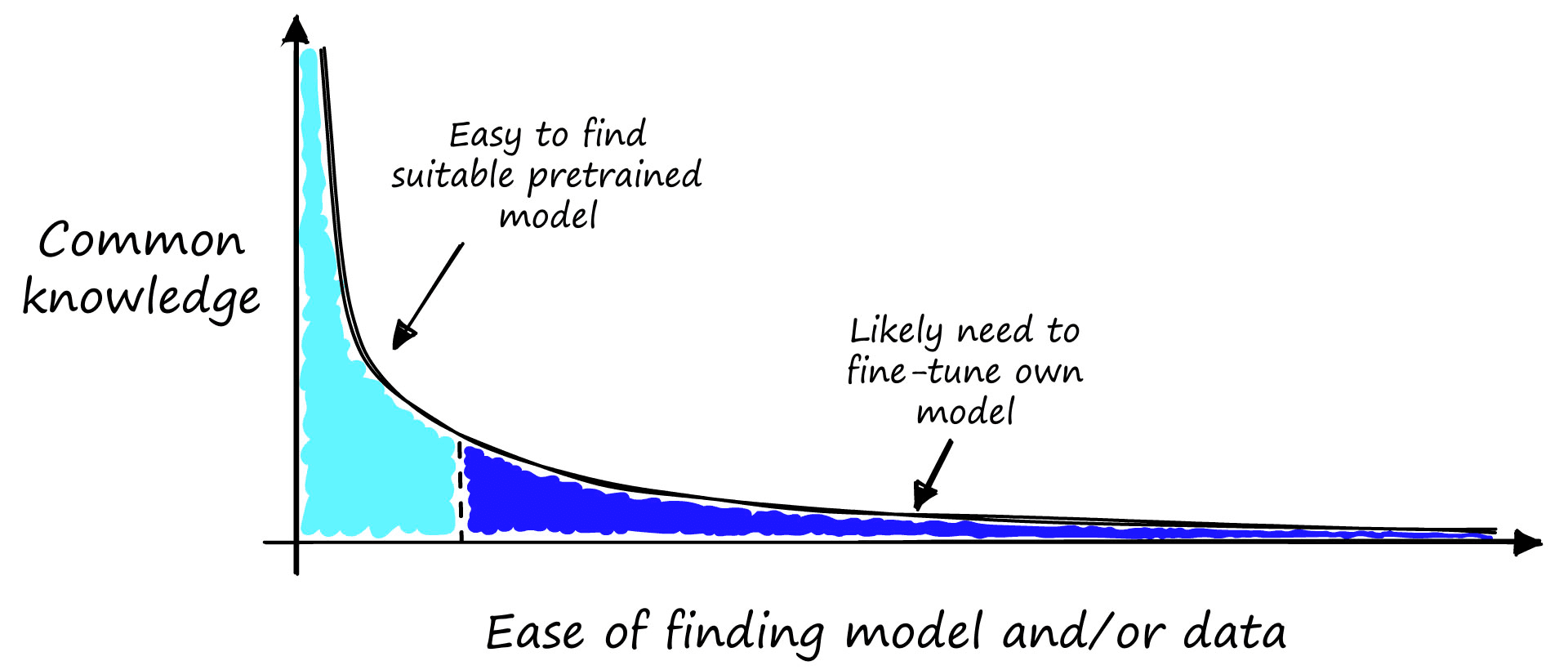
Imagine you are walking down your local high street. You pick a stranger at random and ask them the sort of question that you would expect from your use case. Do you think they would get the answer? If there’s a good chance they will, you might be able to get away with a pretrained model.
On the other hand, if you ask this stranger what the difference is between RoBERTa and DeBERTa, there is a very high chance that they will have no idea what you’re asking. In this case, you will probably need to fine-tune a retriever model.
Fine-Tuning a Retriever
Let’s assume the strangers on the street have no chance of answering our questions. Most likely, a custom retriever model is our best bet. But, how do we train/fine-tune a custom retriever model?
The very first ingredient is data. Our retriever consumes a question and returns relevant contexts to us. For it to do this, it must learn to encode similar question-context pairs into the same vector space.
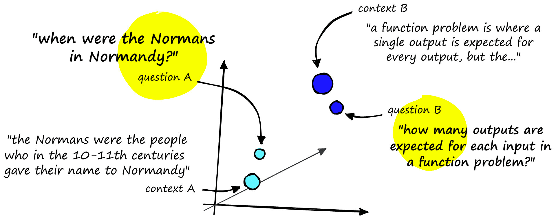
Our first task is to find and create a set of question-context pairs. One of the best-known datasets for this is the Stanford Question Answering Dataset (SQuAD).
Step One: Data
SQuAD is a reading comprehension dataset built from question, context, and answers with information from Wikipedia articles. Let’s take a look at an example.
# install HF datasets library if needed
!pip install datasetsfrom datasets import load_dataset
squad = load_dataset('squad_v2', split='train')
squadDataset({
features: ['id', 'title', 'context', 'question', 'answers'],
num_rows: 130319
})squad[0]{'id': '56be85543aeaaa14008c9063',
'title': 'Beyoncé',
'context': 'Beyoncé Giselle Knowles-Carter (/biːˈjɒnseɪ/ bee-YON-say) (born September 4, 1981) is an American singer, songwriter, record producer and actress. Born and raised in Houston, Texas, she performed in various singing and dancing competitions as a child, and rose to fame in the late 1990s... featured the Billboard Hot 100 number-one singles "Crazy in Love" and "Baby Boy".',
'question': 'When did Beyonce start becoming popular?',
'answers': {'text': ['in the late 1990s'], 'answer_start': [269]}}We first download the squad_v2 dataset via 🤗 Datasets. In the first sample, we can see:
- the title (or topic) of Beyoncé
- the context, a short paragraph from Wikipedia about Beyoncé
- a question, “When did Beyonce start becoming popular?"
- the answer text, “in the late 1990s”, which is extracted from the context
- the answer_start, which is the starting position of the answer within the context string.
The SQuAD v2 dataset contains 130,319 of these samples, more than enough for us to train a good retriever model.
We will be using the Sentence Transformers library to train our retriever model. When using this library, we must format our training data into a list of InputExample objects.
from sentence_transformers import InputExample
from tqdm.auto import tqdm

train = []
for row in tqdm(squad):
    train.append(InputExample(
        texts=[row['question'], row['context']]
))100%|██████████| 130319/130319 [00:08<00:00, 16011.35it/s]
After creating this list of InputExample objects, we need to load them into a data loader. A data loader is commonly used with PyTorch, which Sentence Transformers uses under the hood. Because of this, we can often use the PyTorch DataLoader class.
However, we need to do something slightly different. Our training data consists of positive question-context pairs; positive meaning that every sample in our dataset can be viewed as having a positive or high similarity. There are no negative or dissimilar pairs.
When our data looks like this, one of the most effective training techniques we can use uses the Multiple Negatives Ranking (MNR) loss function. We will not explain MNR loss in this article, but you can learn about it here.
One crucial property of training with MNR loss is that each training batch does not contain duplicate questions or contexts. This is a problem, as the SQuAD data includes several questions for each context. Because of this, if we used the standard DataLoader, there is a high probability that we would find duplicate contexts in our batches.
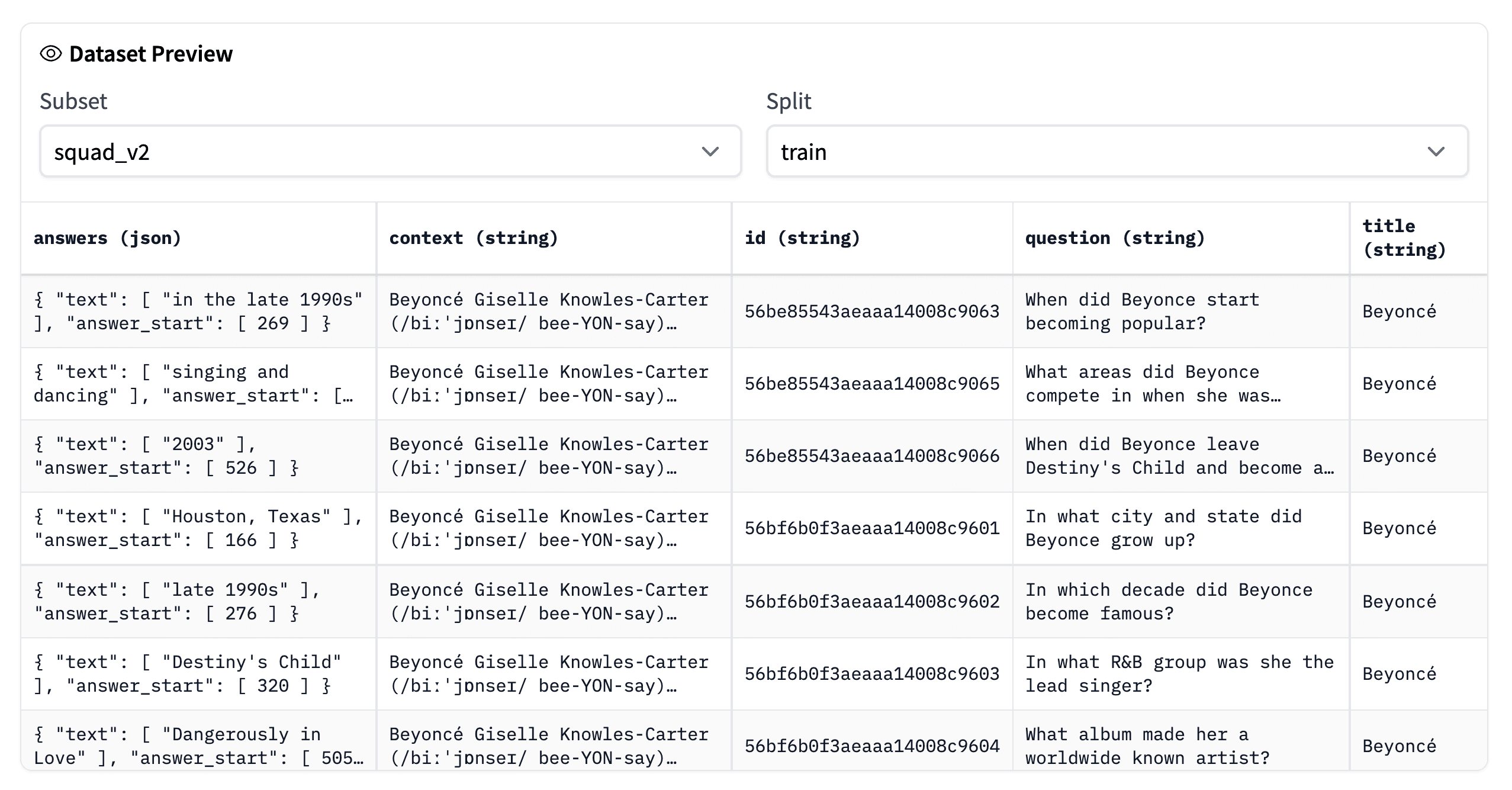
Fortunately, there is an easy solution to this. Sentence Transformers provides a set of modified data loaders. One of those is the NoDuplicatesDataLoader, which ensures our batches contain no duplicates.
from sentence_transformers import datasets

batch_size = 24

loader = datasets.NoDuplicatesDataLoader(
    train, batch_size=batch_size
)
With that, our training data is fully prepared, and we can move on to initializing and training our retriever model.
Step Two: Initialize and Train
Before training our model, we need to initialize it. For this, we begin with a pretrained transformer model from the HuggingFace model hub. A popular choice for sentence transformers is Microsoft’s MPNet model, which we access via microsoft/mpnet-base.
There is one problem with our pretrained transformer model. It outputs many word/token-level vector embeddings. We don’t want token vectors; we need sentence vectors.
We need a way to transform the many token vectors output by the model into a single sentence vector.
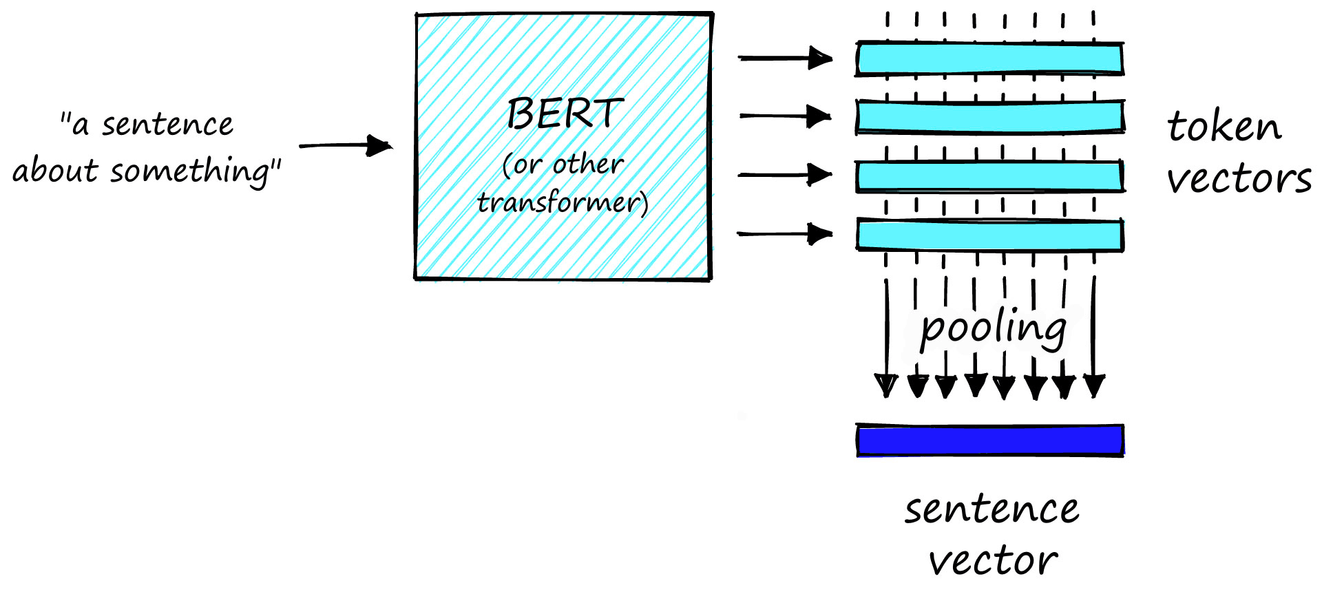
To perform this transformation, we add a mean pooling layer to process the outputs of the transformer model. There are a few different pooling techniques. The one that we will use is mean pooling. This approach will take the many token vectors output by the model and average the activations across each vector dimension to create a single sentence vector.
We can do this via models and SentenceTransformer utilities of the Sentence Transformers library.
from sentence_transformers import models, SentenceTransformer

bert = models.Transformer('microsoft/mpnet-base')
pooler = models.Pooling(
    bert.get_word_embedding_dimension(),
    pooling_mode_mean_tokens=True
)

model = SentenceTransformer(modules=[bert, pooler])

modelSentenceTransformer(
(0): Transformer({'max_seq_length': 512, 'do_lower_case': False}) with Transformer model: MPNetModel
(1): Pooling({'word_embedding_dimension': 768, 'pooling_mode_cls_token': False, 'pooling_mode_mean_tokens': True, 'pooling_mode_max_tokens': False, 'pooling_mode_mean_sqrt_len_tokens': False})
)We have a SentenceTransformer object; a pretrained microsoft/mpnet-base model followed by a mean pooling layer.
With our model defined, we can initialize our MNR loss function.
from sentence_transformers import losses

loss = losses.MultipleNegativesRankingLoss(model)
That is everything we need for fine-tuning the model. We set the number of training epochs to 1; anything more for sentence transformers often leads to overfitting. Another method to reduce the likelihood of overfitting is adding a learning rate warmup. Here, we warmup for the first 10% of our training steps (10% is the go to % for warmup steps; if you find the model is overfitting, try increasing the number).
epochs = 1
warmup_steps = int(len(loader) * epochs * 0.1)

model.fit(
    train_objectives=[(loader, loss)],
    epochs=epochs,
    warmup_steps=warmup_steps,
    output_path='mpnet-mnr-squad2',
    show_progress_bar=True
)Iteration: 100%|██████████| 5429/5429 [28:42<00:00, 3.15it/s]
Epoch: 100%|██████████| 1/1 [28:42<00:00, 1722.72s/it]
We now have an ODQA retriever model saved to the local ./mpnet-mnr-squad2 directory. That’s great, but we have no idea how well the model performs, so our next step is to evaluate model performance.
Retriever Evaluation
Evaluation of retriever models is slightly different from the evaluation of most language models. Typically, we input some text and calculate the error between clearly defined predicted and true values.
For information retrieval (IR), we need a metric that measures the rate of successful vs. unsuccessful retrievals. A popular metric for this is mAP@K. In short, this is an averaged precision value (fraction of retrieved contexts that are relevant) that considers the top K of retrieved results.
The setup for IR evaluation is a little more involved than with other evaluators in the Sentence Transformers library. We will be using the InformationRetrievalEvaluator, and this requires three inputs:
- ir_queries is a dictionary mapping question IDs to question text
- ir_corpus maps context IDs to context text
- ir_relevant_docs maps question IDs to their relevant context IDs
Before we initialize the evaluator, we need to download a new set of samples that our model has not seen before and format them into the three dictionaries above. We will use the SQuAD validation set.
squad_dev = load_dataset('squad_v2', split='validation')
squad_dev[0]{'id': '56ddde6b9a695914005b9628',
'title': 'Normans',
'context': 'The Normans (Norman: Nourmands; French: Normands; Latin: Normanni) were the people who in the 10th and 11th centuries gave their name to Normandy, a region in France... it continued to evolve over the succeeding centuries.',
'question': 'In what country is Normandy located?',
'answers': {'text': ['France', 'France', 'France', 'France'],
'answer_start': [159, 159, 159, 159]}}To create the dictionary objects required by the InformationRetrievalEvaluator, we must assign unique IDs to both contexts and questions. And we need to ensure that duplicate contexts are not assigned different IDs. To handle these, we will first convert our dataset object into a Pandas dataframe.
import pandas as pd

squad_df = pd.DataFrame()
for row in tqdm(squad_dev):
    squad_df = squad_df.append({
        'question': row['question'],
        'context': row['context'],
        'id': row['id']
    }, ignore_index=True)
squad_df.head()100%|██████████| 11873/11873 [00:20<00:00, 576.84it/s]
                                             context  \
0  The Normans (Norman: Nourmands; French: Norman...
1  The Normans (Norman: Nourmands; French: Norman...
2  The Normans (Norman: Nourmands; French: Norman...
3  The Normans (Norman: Nourmands; French: Norman...
4  The Normans (Norman: Nourmands; French: Norman...

                         id                                           question
0  56ddde6b9a695914005b9628               In what country is Normandy located?
1  56ddde6b9a695914005b9629                 When were the Normans in Normandy?
2  56ddde6b9a695914005b962a      From which countries did the Norse originate?
3  56ddde6b9a695914005b962b                          Who was the Norse leader?
4  56ddde6b9a695914005b962c  What century did the Normans first gain their ...
From here, we can quickly drop duplicate contexts with the drop_duplicates method. As we no longer have duplicates, we can append 'con' to each context ID, giving each unique context a unique ID different from any question IDs.
no_dupe = squad_df.drop_duplicates(
    subset='context',
    keep='first'
)
# also drop question column
no_dupe = no_dupe.drop(columns=['question'])
# and give each context a slightly unique ID
no_dupe['id'] = no_dupe['id'] + 'con'
no_dupe.head() context \
0 The Normans (Norman: Nourmands; French: Norman...
9 The Norman dynasty had a major political, cult...
17 The English name "Normans" comes from the Fren...
21 In the course of the 10th century, the initial...
28 Before Rollo's arrival, its populations did no...
id
0 56ddde6b9a695914005b9628con
9 56dddf4066d3e219004dad5fcon
17 56dde0379a695914005b9636con
21 56dde0ba66d3e219004dad75con
28 56dde1d966d3e219004dad8dcon We now have unique question IDs in the squad_df dataframe and unique context IDs in the no_dupe dataframe. Next, we perform an inner join on the context feature to bring these two sets of IDs together and find our question ID to context ID mappings.
squad_df = squad_df.merge(no_dupe, how='inner', on='context')
squad_df.head() context \
0 The Normans (Norman: Nourmands; French: Norman...
1 The Normans (Norman: Nourmands; French: Norman...
2 The Normans (Norman: Nourmands; French: Norman...
3 The Normans (Norman: Nourmands; French: Norman...
4 The Normans (Norman: Nourmands; French: Norman...
id_x \
0 56ddde6b9a695914005b9628
1 56ddde6b9a695914005b9629
2 56ddde6b9a695914005b962a
3 56ddde6b9a695914005b962b
4 56ddde6b9a695914005b962c
question \
0 In what country is Normandy located?
1 When were the Normans in Normandy?
2 From which countries did the Norse originate?
3 Who was the Norse leader?
4 What century did the Normans first gain their ...
id_y
0 56ddde6b9a695914005b9628con
1 56ddde6b9a695914005b9628con
2 56ddde6b9a695914005b9628con
3 56ddde6b9a695914005b9628con
4 56ddde6b9a695914005b9628con We’re now ready to build the three mapping dictionaries for the InformationRetrievalEvaluator. First, we map question/context IDs to questions/contexts.
ir_queries = {
    row['id_x']: row['question'] for i, row in squad_df.iterrows()
}
ir_queries{'56ddde6b9a695914005b9628': 'In what country is Normandy located?',
'56ddde6b9a695914005b9629': 'When were the Normans in Normandy?',
'56ddde6b9a695914005b962a': 'From which countries did the Norse originate?',
...}ir_corpus = {
row['id_y']: row['context'] for i, row in squad_df.iterrows()
}
ir_corpus{'56ddde6b9a695914005b9628con': 'The Normans (Norman: Nourmands; French: Normands; Latin: Normanni) were the people... to evolve over the succeeding centuries.',
'56dddf4066d3e219004dad5fcon': 'The Norman dynasty had a major political, cultural and military impact on medieval... north Africa and the Canary Islands.',
'56dde0379a695914005b9636con': 'The English name "Normans" comes from the French words Normans/Normanz, plural of... 9th century) to mean "Norseman, Viking".',
...}And then map question IDs to a set of relevant context IDs. For the SQuAD data, we only have many-to-one or one-to-one question ID to context ID mappings, but we will write our code to additionally handle one-to-many mappings (so we can handle other, non-SQuAD datasets).
ir_relevant_docs = {key: [] for key in squad_df['id_x'].unique()}
for i, row in squad_df.iterrows():
    # we append in the case of a question ID being connected to
    # multiple context IDs
    ir_relevant_docs[row['id_x']].append(row['id_y'])
# this must be in format {question_id: {set of context_ids}}
ir_relevant_docs = {key: set(values) for key, values in ir_relevant_docs.items()}
ir_relevant_docs{'56ddde6b9a695914005b9628': {'56ddde6b9a695914005b9628con'},
'56ddde6b9a695914005b9629': {'56ddde6b9a695914005b9628con'},
'56ddde6b9a695914005b962a': {'56ddde6b9a695914005b9628con'},
...}Our evaluator inputs are ready, so we initialize the evaluator and then evaluate our model.
ir_eval = InformationRetrievalEvaluator(
    ir_queries, ir_corpus, ir_relevant_docs
)ir_eval(model)0.7414982703270794We return a mAP@K score of 0.74, where @K is 100 by default. This performance is comparable to other state-of-the-art retriever models. Performing the same evaluation with the multi-qa-mpnet-base-cos-v1 returns a mAP@K score of 0.76, just two percentage points greater than our custom model.
qa = SentenceTransformer('multi-qa-mpnet-base-cos-v1')

ir_eval(qa)0.7610692295248334Of course, if your target domain was SQuAD data, the pretrained multi-qa-mpnet-base-cos-v1 model would be the better model. But if you have your own unique dataset and domain. A custom model fine-tuned on that domain will very likely outperform existing models like multi-qa-mpnet-base-cos-v1 in that domain.
Storing the Vectors
We have our retriever model, we’ve evaluated it, and we’re happy with its performance. But we don’t know how to use it.
When you perform a Google search, Google does not look at the whole internet, encode all of that information into vector embeddings, and then compare all of those vectors to your query vector. We would be waiting a very long time to return results if that were the case.
Instead, Google has already searched for, collected, and encoded all of that data. Google then stores those encoded vectors in some sort of vector database. When you query now, the only thing Google needs to encode is your question.
Taking this a step further, comparing your query vector to all vectors indexed by Google (which represent the entire Google-accessible internet) would still take an incredibly long time. We refer to this accurate but inefficient comparison of every single vector as an exhaustive search.
For big datasets, an exhaustive search is too slow. The solution to this is to perform an approximate search. An approximate search allows us to massively reduce our search scope to a smaller but (hopefully) more relevant sub-section of the index. Making our search times much more manageable.
The Pinecone vector database is a straightforward and robust solution that allows us to (1) store our context vectors and (2) perform an accurate and fast approximate search. These are the two elements we need for a promising ODQA pipeline.
Again, we need to work through a few steps to set up our vector database.
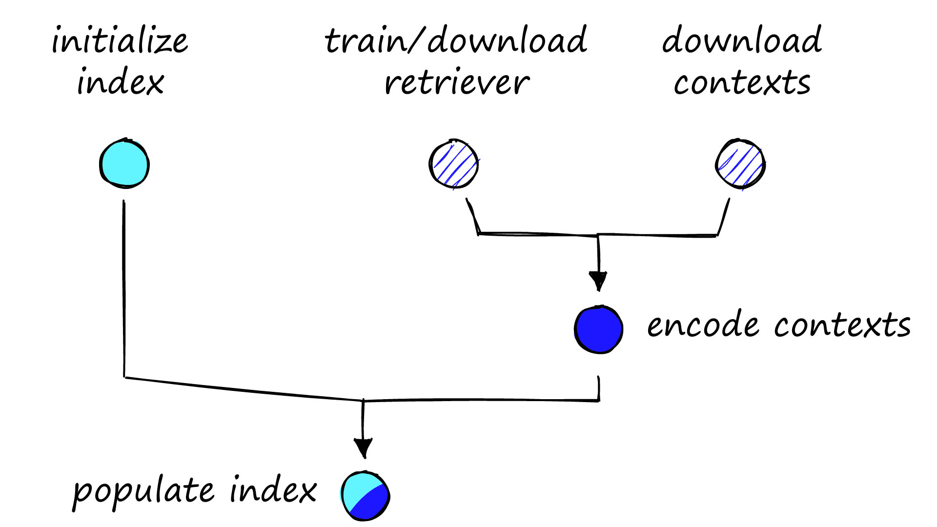
After working through each of those steps, we will be ready to begin retrieving relevant contexts.
Encoding Contexts
We have already created our retriever model, and during the earlier evaluation step, we downloaded the SQuAD validation data. We can use this same validation data and encode all unique contexts.
unique_contexts = []
unique_ids = []

# make list of IDs that represent only first instance of
# each context
for row in squad_dev:
    if row['context'] not in unique_contexts:
        unique_contexts.append(row['context'])
        unique_ids.append(row['id'])

# now filter out any samples that aren't included in unique IDs
squad_dev = squad_dev.filter(lambda x: True if x['id'] in unique_ids else False)
squad_devDataset({
features: ['id', 'title', 'context', 'question', 'answers'],
num_rows: 1204
})# and now encode the unique contexts
squad_dev = squad_dev.map(lambda x: {
'encoding': model.encode(x['context']).tolist()
}, batched=True, batch_size=4)
squad_dev100%|██████████| 301/301 [20:18<00:00, 4.05s/ba]
Dataset({
    features: ['answers', 'context', 'encoding', 'id', 'question', 'title'],
    num_rows: 1204
})
After removing duplicate contexts, we’re left with 1,204 samples. It is a tiny dataset but large enough for our example.
Initializing the Index
Before adding the context vectors to our index, we need to initialize it. Fortunately, Pinecone makes this very easy. We start by installing the Pinecone client if required:
!pip install pinecone-client
Then we initialize a connection to Pinecone. For this, we need a free API key.
import pineconeAPI_KEY = 'YOUR_API_KEY'
pinecone.init(api_key=API_KEY, environment='YOUR_ENV')
# (find env next to API key in consoleWe then create a new index with pinecone.create_index. Before initializing the index, we should check that the index name does not already exist (which it will not if this is your first time creating the index).
# check if index already exists, if not we create it
if 'squad-index' not in pinecone.list_indexes():
    pinecone.create_index(
        name='squad-index', dimension=model.get_sentence_embedding_dimension(), metric='cosine'
)# we use this to get required index dims
model.get_sentence_embedding_dimension()768When creating a new index, we need to specify the index name, and the dimensionality of vectors to be added. We either check our encoded context vectors’ dimensions directly or find the dimension attribute within the retriever model (as shown above).
Populating the Index
After creating both our index and the context vectors, we can go ahead and upsert (upload) the vectors into our index.
# initialize connection to the new index
index = pinecone.Index('squad-index')from tqdm.auto import tqdm # progress bar
upserts = [(v['id'], v['encoding'], {'text': v['context']}) for v in squad_dev]
# now upsert in chunks
for i in tqdm(range(0, len(upserts), 50)):
i_end = i + 50
if i_end > len(upserts): i_end = len(upserts)
index.upsert(vectors=upserts[i:i_end])100%|██████████| 25/25 [00:13<00:00, 1.91it/s]
Pinecone expects us to upsert data in the format:
vectors =
[
(id_0, vector_0, metadata_0),
(id_1, vector_1, metadata_1)
]
Our IDs are the unique alphanumeric identifiers that we saw earlier in the SQuAD data. The vectors are our encoded context vectors formatted as lists; the metadata is a dictionary that allows us to store extra information in a key-value format.
Using the metadata field, Pinecone allows us to create complex or straightforward metadata filters to target our search scope to specific numeric ranges, categories, and more.
Once the upsert is complete, the retrieval components of our ODQA pipeline are ready to go, and we can begin asking questions.
Making Queries
With everything set up, querying our retriever-vector database pipeline is pretty straightforward. We first define a question and encode it as we did for our context vectors before.
query = "When were the Normans in Normandy?"
xq = model.encode([query]).tolist()
After creating our query vector, we pass it to Pinecone via the index.query method, specify how many results we’d like to return with top_k, and include_metadata so that we can see the text associated with each returned vector.
xc = index.query(xq, top_k=2, include_metadata=True)
xc{'results': [{'matches': [{'id': '56dddf4066d3e219004dad5f',
'metadata': {'text': 'The Norman dynasty had a '
'major political, cultural and '
'military impact on medieval '
'Europe and even the Near '
'East. The Normans were famed '
'for their martial spirit and '
'eventually for their '
'...'
'Ireland, and to the coasts of '
'north Africa and the Canary '
'Islands.'},
'score': 0.678345382,
'values': []},
{'id': '56ddde6b9a695914005b9628',
'metadata': {'text': 'The Normans (Norman: '
'Nourmands; French: Normands; '
'Latin: Normanni) were the '
'people who in the 10th and '
'11th centuries gave their '
'name to Normandy, a region in '
'France. They were descended '
'...'
'of the 10th century, and it '
'continued to evolve over the '
'succeeding centuries.'},
'score': 0.667023182,
'values': []}],
'namespace': ''}]}We return the correct context as our second top result in this example. The first result is relevant in the context of Normans and Normandy, but it does not answer the specific question of when the Normans were in Normandy.
Let’s try a couple more questions.
xq = model.encode([
    "How many outputs are expected for each input in a function problem?"
]).tolist()
index.query(xq, top_k=5, include_metadata=True){'results': [{'matches': [{'id': '56e19724cd28a01900c679f6',
'metadata': {'text': 'A function problem is a '
'computational problem where a '
'single output (of a total '
'function) is expected for '
'every input, but the output '
'...'
'and the integer factorization '
'problem.'},
'score': 0.7924698,
'values': []},
{'id': '56e17a7ccd28a01900c679a1',
'metadata': {'text': 'A computational problem can '
'be viewed as an infinite '
'...'},
'score': 0.662115633,
'values': []},
{'id': '56e1a0dccd28a01900c67a2e',
'metadata': {'text': 'It is tempting to think that '
'the notion of function '
'...'},
'score': 0.615972638,
'values': []},
{'id': '56e19557e3433e1400422fee',
'metadata': {'text': 'An example of a decision '
'problem is the following. The '
'...'},
'score': 0.599050403,
'values': []},
{'id': '56e190bce3433e1400422fc8',
'metadata': {'text': 'Decision problems are one of '
'the central objects of study '
'...'},
'score': 0.593822241,
'values': []}],
'namespace': ''}]}For this question, we return the correct context as the highest result with a much higher score than the remaining samples.
xq = model.encode([
    "Who used Islamic, Lombard, etc construction techniques in the Mediterranean?"
]).tolist()
index.query(xq, top_k=5, include_metadata=True){'results': [{'matches': [{'id': '56de4b074396321400ee2793',
'metadata': {'text': 'In England, the period of '
'...'
'the Early Gothic. In southern '
'Italy, the Normans '
'incorporated elements of '
'Islamic, Lombard, and '
'Byzantine building techniques '
'...'},
'score': 0.604390621,
'values': []},
{'id': '56de51244396321400ee27ef',
'metadata': {'text': 'In Britain, Norman art '
'primarily survives as '
'...'},
'score': 0.487686485,
'values': []},
{'id': '56de4a89cffd8e1900b4b7bd',
'metadata': {'text': 'Norman architecture typically '
'stands out as a new stage in '
'...'},
'score': 0.451720327,
'values': []},
{'id': '56de4b5c4396321400ee2799',
'metadata': {'text': 'In the visual arts, the '
'Normans did not have the rich '
'...'},
'score': 0.343783677,
'values': []},
{'id': '57287c142ca10214002da3d0',
'metadata': {'text': 'The Yuan undertook extensive '
'public works. Among Kublai '
'...'},
'score': 0.335578799,
'values': []}],
'namespace': ''}]}We return the correct context in the first position. Again, there is a good separation between sample scores of the correct context and other contexts.
That’s it for this guide to fine-tuning and implementing a custom retriever model in an ODQA pipeline. Now we can implement two of the most crucial components in ODQA: enabling a more human and natural approach to information retrieval.
One of the most incredible things about ODQA is how widely applicable it is. Organizations across almost every industry have the opportunity to benefit from more intelligent and efficient information retrieval.
Any organization that handles unstructured information such as word documents, PDFs, emails, and more has a clear use case: freeing this information and enabling easy and natural access through QA systems.
Although this is the most apparent use case, there are many more, whether it be an internal efficiency speedup or a key component in a product (as with Google search). The opportunities are both broad and highly impactful.
References
[1] N. Reimers, Neural Search for Low Resource Scenarios (2021), YouTube
S. Sawtelle, Mean Average Precision (MAP) For Recommender Systems (2016), GitHub